JFL210 SIGNAL PROCESSING APPLICATION GUIDE

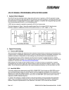
1. System Block Diagram

The JFL210 has two powering modes: single-amp and bi-amp. In general, a JFL210 operated in singleamp mode only requires a high pass filter for low frequency excursion protection. The high pass filter may be implemented in a Digital Signal Processor (DSP), equaliser, or amplifier with integrated high pass filter.

The recommended filter is 60 Hz, 12 to 24 dB Butterworth.

A DSP with two outputs is required to operate the JFL210 in bi-amp mode.

The block diagrams in Figure 1 show the possible signal flows for a single JFL210. Use the same processor outputs for additional JFL210s on the same mix bus, i.e. “Left”, “Right”, or “Fill”.

DSP

EQ

HPF

FULL

HF

LF

DSP

PEQ

HF

HF

LF

JFL210

LF

JFL210

JFL210 BI-AMP MODE JFL210 SINGLE-AMP MODE

2. Signal Processing

Figure 1

2.1 Factory DSP Settings

JFL210 processor settings are determined from extensive measurements in laboratory environments and in typical venues. Loudspeaker performance in terms of frequency response, beamwidth consistency, and wavefront coherency is dependent on these settings; they should thus be fully implemented “as is.”

The highest performance will be achieved using Gunness Focusing™-enabled Greyboxes in EAW’s

UX8800 Digital Signal Processor. JFL Greyboxes may be found in the UX8800 Greyboxes installer that is available for download from http://www.eaw.com/downloads/ .

EAW settings will normally provide excellent results in a variety of venues, but parametric or graphic equalisation may be used to adjust JFL Series tonality to best suit particular programs, venues, or user tastes. This EQ should be applied before the output bandpass processing, e.g. the input filters of a DSP.

2.2 Non-EAW DSPs

The factory settings were determined using EAW’s UX8800 DSP. Even though non-EAW DSPs can be set to numerically equal values, the actual transfer function (magnitude and phase) of the processing depends on the particular digital processor. The reason is that different algorithms can be and are used to implement the same processing functions. If you use a non-EAW DSP, care must be paid to match its response to EAW’s intended response.

To assist in this endeavor, transfer functions of JFL210 processing curves accompany this application guide. They are formatted as Reference Trace files for direct import into EAW Smaart ® measurement software. Graphical representations of the Reference Trace files in PDF format are also included.

Page 1 of 7 RD0482 (A) JFL210 Signal Processing App Guide Oct 2008

2.2.1 Equalisation Filter Width Specifications

EAW specifies equalisation filter width in terms of Quality factor – more commonly known as “Q”. Some DSP manufacturers instead specify filter width in terms of bandwidth – or BW. Converting between Q and BW is a relatively simple affair; however, several methodologies exist for doing so. Sections 4 thru 6 – JFL210

Processor Settings includes conversions for the two most popular methods: bilinear transform (or BZT) and

Orfanidis. These are labeled “BW1” and “BW2” respectively. Consult your DSP manufacturer to determine which method they use. A (very) brief discussion of BZT implementation may be found in the technical paper

“BZT Implementation of Parametric Filters”, available for download at http://www.eaw.com/downloads/ . The

Orfanidis method is outlined in the following AES paper:

S.J. Orfanidis, "Digital Parametric Equalizer Design with Prescribed Nyquist-Frequency Gain", Journal of the

Audio Engineering Society, vol. 45, No. 6, 1997 June

2.3 User Adjustments

2.3.1 JFL210 HF Shading – Single-Amp Mode

A three-position, rear panel switch labeled “HF

Shading” is active when with the JFL210 is operated in Single-amp Mode. This switch is much more than a simple HF gain control. Instead, each of the three positions employs sophisticated high frequency shading to tailor the JFL210’s high frequency response for different applications: Single Box, Multi

Box, and Long Throw.

• Single Box

This switch position provides an HF character that is suitable for use with a single JFL210 that is not used in an array. It may also be used to attenuate the HF response of the bottom, or

“nearfield”, loudspeaker in a large array. The latter application is noted where appropriate in

Section 4 – JFL210 Single-Amp Processor

Settings. Figure 3 illustrates the typical axial response of one JFL210 set to Single Box mode.

• Multi Box

This switch position provides an HF character that is suitable for use with multiple, arrayed

JFL210s in short to medium throw applications – approximately 1 to 18 meters / 3 to 60 feet. It provides a 2 octave wide boost centered around

4 kHz. Though this may appear odd at first glance, note that the low and low/mid frequency output of an array increases as JFL210 are added. This behavior in large part mimics a 1st order shelf filter. The 4 kHz boost is designed to neatly integrate with the low frequency shelf while not excessively boosting very high frequencies.

The net effect can be seen in Figure 4. The brown and red curves illustrate the change in HF response when Multi Box mode is engaged on a single JFL210. The green curve illustrates the response of two JFL210 set to Multi Box mode.

Figure 2

Figure 3

Page 2 of 7

Figure 4

RD0482 (A) JFL210 Signal Processing App Guide Oct 2008

• Long Throw

This switch position provides an HF character that is suitable for use with multiple, arrayed JFL210s in long throw applications – approximately 18 to 30 meters / 60 to 100 feet. Using this switch position will maintain tonal balance at long distances by adding compensation to those frequencies that suffer attenuation due to air loss. The magenta curve in Figure 5 illustrates typical high frequency air loss at 30 meters, while the blue curve shows the compensation filter applied to a JFL210 when the Long Throw switch is engaged. The net result may be seen in Figure 6: the green curve is the magnitude response of two JFL210 set to Multi Box mode, while the purple curve is the magnitude response of two JFL210 set to

Long Throw mode.

Figure 5 Figure 6

In an array where some JFL210s are used for short to medium distances and others are used for long distances, it is appropriate to mix Single-Box, Multi Box, and Long Throw settings to taper the HF response throughout an array. Please see Note 5 in Section 4 – JFL210 Single-Amp Processor Settings for recommended progressions.

2.3.2 JFL210 HF Shading – Bi-Amp Mode

The single-amp HF shading toggle switch described in Section 2.3.1 is disabled when the JFL210 is operated in bi-amp powering mode. HF Shading functions are instead replicated in DSP. In an array where some JFL210s are used for short to medium distances and others are used for long distances, it is appropriate to taper the HF response throughout an array by using additional HF DSP outputs and zoning

HF drivers on different amplifier channels. Please see Notes in Section 4 – JFL210 Processor Settings for recommended progressions.

2.4 Array Low Frequency Settings

Low and low/mid frequency Sound Pressure Level (SPL) will increase as JFL210 loudspeakers are added to an array. Complementary, inverse filters may be applied in DSP to restore the desired system tonal balance. Typically these “array” filters are implemented using the input equalisation section of a DSP.

However some users may wish to reserve all input equalisation for guest audio engineers. In this case the array filters may be applied to the DSP’s output equalisation sections. Note that the array filters span the

JFL210’s LF/HF crossover point, thus they should be applied to LF and HF output band passes so that the crossover’s phase integrity is maintained. Recommended array low frequency compensation filters are noted with italics in Sections 4 & 6 – JFL210 Processor Settings.

Page 3 of 7 RD0482 (A) JFL210 Signal Processing App Guide Oct 2008

3. Amplifier Gain Settings

In order for EAW signal processing to function properly for multi-amplified loudspeakers it is critical that all amplifiers for all passbands be set to the same voltage gain, regardless of the amplifiers’ power output ratings. NOTE: The same voltage gain does NOT mean the same input sensitivity, but the same input to output voltage ratio. Voltage gain is normally specified in dB units (i.e. 32 dB) but may also be expressed as a multiplier (e.g. x40, which is equivalent to a 40:1 ratio, or 32 dB). Consult your amplifier manufacturer if this cannot be readily determined.

3.1 Amplifier Gain Settings in UX8800 Processor

Greybox processing in EAW’s UX8800 DSP automatically adjusts output levels to compensate for amplifiers with differing voltage gains. The user need only enter the gain of the amplifier connected to each Greybox output leg during system setup; the processor will do the rest of the work.

3.2 Amplifier Gains in Other Processors

If your amplifiers do not meet the constant voltage gain criteria, the DSP’s output gains may be trimmed by the user to “equalise” amplifier gains. The table below can be used for guidance. Choose a reference amplifier gain in the left-most column and read across that row for appropriate processor gain adjustments .

Step 2: Add/Subtract Value from Processor Output for Differing Amplifier Gain(s)

26 27 28 29 30 31 32 33 34 35 36 37 38 39 40 41 42

Step 1:

Select

Reference

Amplifier

Gain

26 0 -1 -2 -3 -4 -5 -6 -7 -8 -9 -10 -11 -12 -13 -14 -15 -16

27 1 0 -1 -2 -3 -4 -5 -6 -7 -8 -9 -10 -11 -12 -13 -14 -15

28 2 1 0 -1 -2 -3 -4 -5 -6 -7 -8 -9 -10 -11 -12 -13 -14

29 3 2 1 0 -1 -2 -3 -4 -5 -6 -7 -8 -9 -10 -11 -12 -13

30 4 3 2 1 0 -1 -2 -3 -4 -5 -6 -7 -8 -9 -10 -11 -12

31 5 4 3 2 1 0 -1 -2 -3 -4 -5 -6 -7 -8 -9 -10

32 6 5 4 3 2 1 0 -1 -2 -3 -4 -5 -6 -7 -8 -9 -10

33 7 6 5 4 3 2 1 0 -1 -2 -3 -4 -5 -6 -7 -8 -9

34 8 7 6 5 4 3 2 1 0 -1 -2 -3 -4 -5 -6 -7 -8

35* 9 8 7 6 5 4 3 2 1 0 -1 -2 -3 -4 -5 -6 -7

36 10 9 8 7 6 5 4 3 2 1 0 -1 -2 -3 -4 -5 -6

37 11

38 12 10 9 8 7 6 5 4 3 2 1 0 -1 -2 -3 -4

39 13

40 14 13 12 11 10 9 8 7 6 5 4 3 2 1 0 -1 -2

41 15 14 13 12 11 10 9 8 7 6 5 4 3 2 1 0 -1

42 16 15 14 13 12 11 10 9 8 7 6 5 4 3 2 1 0

* 35 dB is the Reference Voltage Gain in the examples below.

Generally speaking, for best signal-to-noise performance choose the amplifier with the lowest voltage gain and “match” the other amplifier to it by subtracting gain from the other processor output channel.

For example:

LF Amplifier

HF Amplifier

Voltage Gain Proc Output Gain

39 -4

35* 0

Page 4 of 7 RD0482 (A) JFL210 Signal Processing App Guide Oct 2008

4. JFL210 Single-Amp Processor Settings

OUTPUT

GAIN

DELAY

POLARITY

HPF

(2)

LPF

PEQ1

(1)

Name

(dB)

(ms)

Type

Freq (Hz)

Type

Freq (Hz)

Type

PEQ2

(1)

Freq (Hz)

Level (dB)

Q

BW1 / BW2

Type

Freq (Hz)

Level (dB)

Q

BW1 / BW2

JFL210 x1

SNGL NEAR

(3)

Full Range

0.0

0.000

Normal

12 dB Butterworth

60

Thru

6 dB HiShelf

2239

-2.0

JFL210 x1-3

SNGL

(4)

Full Range

0.0

0.000

Normal

12 dB Butterworth

60

Thru

JFL210 x4-6

SNGL

(5)

Full Range

0.0

0.000

Normal

12 dB Butterworth

60

Thru

6 dB LoShelf

1155

-5.0

Parametric

794

1.5

1.26

0.79 / 1.13

Notes

(1) PEQ filters may be applied to input or output processing.

(2) To use JFL210 with a subwoofer set its High Pass Filter and the subwoofer's Low Pass Filter to 100

Hz, 24 dB Linkwitz-Riley.

(3) JFL210 x1 SNGL NEAR - Use for front or side fill applications where typical listener distances are <2 meters. Set HF Shading switch to "Single Box".

(4) JFL210 x1-3 SNGL - Set HF Shading switch to "Single Box" for 1x JFL210 and "Multi Box" for 2-3x

JFL210.

(5) JFL210 x4-6 SNGL - Use HF Shading switches to taper HF response throughout an array.

Recommended top-to-bottom progressions are:

4x JFL210 5x JFL210 6x JFL210

Long Throw Long Throw Long Throw

Multi Box Long Throw Long Throw

Page 5 of 7 RD0482 (A) JFL210 Signal Processing App Guide Oct 2008

OUTPUT

GAIN

DELAY

POLARITY

HPF

(1)

LPF

PEQ1

PEQ2

Name

(dB)

(ms)

Type

Freq (Hz)

Type

Freq (Hz)

Type

Freq (Hz)

Level (dB)

Q

BW1 / BW2

Type

Freq (Hz)

PEQ3

PEQ4

PEQ5

Level (dB)

Q

BW1 / BW2

Type

Freq (Hz)

Level (dB)

Q

BW1 / BW2

Type

Freq (Hz)

Level (dB)

Q

BW1 / BW2

Type

Freq (Hz)

Level (dB)

Q

BW1 / BW2

5. JFL210 Bi-Amp Processor Settings – Part 1

JFL210 x1 BI

(2)

Low

4.0

0.371

Normal

High

-4.0

0.000

Invert

12 dB Butterworth 24 dB Butterworth

60 772

24 dB Butterworth

631

Thru

Parametric

211

-3.0

2.00

0.50 / 0.80

Parametric

473

-4.5

2.82

Parametric

1090

2.5

4.00

0.25 / 0.38

Parametric

1995

-9.5

1.00

0.35 / 0.64

Parametric

631

-3.0

3.55

0.28 / 0.45

Parametric

188

-3.0

7.94

0.13 / 0.20

1.22 / 2.29

Parametric

5788

-2.5

3.00

0.33 / 0.51

Parametric

10000

-2.0

2.24

0.45 / 0.66

JFL210 x1 BI NEAR

(2)(3)

Low

4.0

0.371

Normal

High

-4.0

0.000

Invert

12 dB Butterworth 24 dB Butterworth

60 772

24 dB Butterworth

631

Thru

Parametric

211

-3.0

2.00

0.50 / 0.80

Parametric

473

-4.5

2.82

Parametric

1090

2.5

4.00

0.25 / 0.38

Parametric

1995

-9.5

1.00

0.35 / 0.64

Parametric

631

-3.0

3.55

0.28 / 0.45

Parametric

188

-3.0

7.94

0.13 / 0.20

1.22 / 2.29

Parametric

5788

-2.5

3.00

0.33 / 0.51

Parametric

10000

-2.0

2.24

0.45 / 0.66

6 dB HiShelf

2239

-2.0

Notes

(1) To use JFL210 with a subwoofer set its LF High Pass Filter and the subwoofer's Low Pass Filter to

100 Hz, 24 dB Linkwitz-Riley.

(2) DSP settings are equivalent to single-amp Single Box mode.

(3) JFL210 x1 BI NEAR - Use for front or side fill applications where typical listener distances are <2 meters. Set HF Shading switch to "Single Box".

Page 6 of 7 RD0482 (A) JFL210 Signal Processing App Guide Oct 2008

OUTPUT

GAIN

DELAY

POLARITY

HPF

(2)

LPF

PEQ1

PEQ2

PEQ3

PEQ4

Name

(dB)

(ms)

Type

Freq (Hz)

Type

Freq (Hz)

Type

Freq (Hz)

Level (dB)

Q

BW1 / BW2

Type

Freq (Hz)

Level (dB)

Q

BW1 / BW2

Type

Freq (Hz)

Level (dB)

Q

BW1 / BW2

Type

Freq (Hz)

Level (dB)

Q

BW1 / BW2

PEQ5

(1)

PEQ6

(1)

Type

Freq (Hz)

Level (dB)

Q

BW1 / BW2

Type

Freq (Hz)

Level (dB)

Q

BW1 / BW2

6. JFL210 Bi-Amp Processor Settings – Part 2

JFL210 x2-3 BI

(3)

Low

4.0

0.371

Normal

High

-4.0

0.000

Invert

12 dB Butterworth 24 dB Butterworth

60

24 dB Butterworth

631

Parametric

211

-3.0

2.00

0.50 / 0.80

Parametric

473

-4.5

2.82

0.35 / 0.64

Parametric

631

-3.0

3.55

0.28 / 0.45

Parametric

188

-3.0

7.94

0.13 / 0.20

772

Thru

Parametric

1090

2.5

4.00

0.25 / 0.38

Parametric

1995

-9.5

1.00

1.22 / 2.29

Parametric

5788

-2.5

3.00

0.33 / 0.51

Parametric

10000

-2.0

2.24

0.45 / 0.66

6 dB LoShelf

1155

-5.0

6 dB LoShelf

1155

-5.0

JFL210 x4-6 BI

(3)(4)

Low

4.0

0.371

Normal

High

-4.0

0.000

Invert

12 dB Butterworth 24 dB Butterworth

60

24 dB Butterworth

631

Parametric

211

-3.0

2.00

0.50 / 0.80

Parametric

473

-4.5

2.82

0.35 / 0.64

Parametric

631

-3.0

3.55

0.28 / 0.45

Parametric

188

-3.0

7.94

0.13 / 0.20

772

Thru

Parametric

1090

2.5

4.00

0.25 / 0.38

Parametric

1995

-9.5

1.00

1.22 / 2.29

Parametric

5788

-2.5

3.00

0.33 / 0.51

Parametric

10000

-2.0

2.24

0.45 / 0.66

6 dB LoShelf

1585

-7.0

6 dB LoShelf

1585

-7.0

Parametric

244

-3.0

0.34

2.99 / 4.78

Parametric

244

-3.0

0.34

2.99 / 4.78

Notes

(1) PEQ5 & PEQ6 filters are array low frequency compensation settings and may be applied to input or output processing - see Section 2.4 in this guide.

(2) To use JFL210 with a subwoofer set its LF High Pass Filter and the subwoofer's Low Pass Filter to

100 Linkwitz-Riley.

(3) DSP settings are equivalent to single-amp Multi Box mode. To approximate Single Box and/or Long

Throw modes insert the following filters on the HF channel(s):

Single Box: 5 kHz, -3.0 dB, 1.20 Q (0.83 / 1.33 BW)

Long Throw: 10 kHz, +3 dB, 1.00 Q (1.00 / 1.60 BW)

(4) HF response may be tapered throughout the array by zoning HF drivers on different amp channels and using additional DSP outputs. See Single-Amp Settings, Note 5 for recommended progressions.

Page 7 of 7 RD0482 (A) JFL210 Signal Processing App Guide Oct 2008